14  From super‑k‑mers to hyper-k-mers

Note

This chapter is adapted from (Martayan et al., 2025), accepted to RECOMB 2025 and to be published.

Lucas Robidou and I contributed equally to this work.

The previous chapters built k‑mer dictionaries on top of contiguous super‑k‑mers, one bucket per minimizer. At the k‑mer sizes most prior work is calibrated for, around k = 31, the per-k‑mer cost of this layout is moderate. It degrades as k grows: each super‑k‑mer carries k - 1 bases of overlap with each of its two neighbors, so a super‑k‑mer representation asymptotes to 6 bits per nucleotide as discussed in Section 4.3, three times the 2-bit lower bound. Static representations such as unitigs and eulertigs do reach 2 bits per nucleotide, but they are built once from a finalized k‑mer set, require a separate counting pass, and dissolve the per-minimizer partitioning that the structures of Chapter 13 rely on for cache-friendly indexing and load balancing.

This regime of large k‑mer sizes is becoming practically relevant, as long-read technologies now reach error rates below 1% for Oxford Nanopore (Sereika et al., 2022) and 0.1% for PacBio HiFi (Bankevich et al., 2022), which makes k‑mer sizes in the hundreds tractable and useful for genome assembly, pangenomic comparisons, and fine-grained k‑mer analyses.

In this chapter, we introduce a representation called hyper‑k‑mers that aims to keep the streaming, partitioned nature of super‑k‑mers while approaching the asymptotic efficiency of static representations. The core idea, developed formally in Section 14.2, is to share each k - 1 base overlap between consecutive super‑k‑mers instead of duplicating it on each side, bringing the cost from 6 down to 4 bits per nucleotide at large k.

We put hyper‑k‑mers to work in KFC, a streaming k‑mer counter available at https://github.com/lrobidou/KFC that uses hyper‑k‑mers as primary storage. We describe the counting algorithm in Section 14.3 and compare KFC against existing k‑mer counters in Section 14.4.

14.1 Space analysis of super‑k‑mers and closed syncmers

We use the notation of Chapter 4 throughout: S is a random genomic string over \Sigma = \{A, C, G, T\} with k‑mer size k, minimizer size m < k, window size w = k - m + 1, and minimizer scheme density d, with random minimizers satisfying d = 2 / (w + 1). We add one new notion, the overlap between consecutive super‑k‑mers.

Definition 14.1 (Overlap of consecutive super‑k‑mers) Given two consecutive super‑k‑mers u and v, we define the overlap of u and v, denoted \operatorname{ov}(u, v), as the k - 1 bases shared by the rightmost k‑mer of u and the leftmost k‑mer of v.

This section establishes the asymptotic space cost of super‑k‑mers and closed syncmers, the two reference points that the hyper‑k‑mer analysis in Section 14.2 compares against. Super‑k‑mers are the direct baseline that hyper‑k‑mers improve on. Closed syncmers, while not a stand-alone k‑mer-set representation, are included as a comparison point: they pave sequences better than minimizer-based sampling (Edgar, 2021; Shibuya et al., 2022) and reach 4 bits per nucleotide.

14.1.1 Super‑k‑mers

Lemma 14.1 (Average number of super‑k‑mers) Given a random string S, the expected number of super‑k‑mers is (|S| - m + 1) \times d.

Proof. By definition of the density d, the expected number of minimizers is (|S| - m + 1) \times d. Since each minimizer corresponds to one super‑k‑mer, the expected number of super‑k‑mers is the same.

Lemma 14.2 (Average length of super‑k‑mers) Given a random string S, the average length of a super‑k‑mer is \frac{|S| - k + 1}{(|S| - m + 1) \times d} + k - 1. In particular, it approaches \frac{1}{d} + k - 1 as |S| \to +\infty.

Proof. By Lemma 14.1, there are (|S| - m + 1) \times d super‑k‑mers on average. Since there are |S| - k + 1 k‑mers in S, each super‑k‑mer contains \frac{|S| - k + 1}{(|S| - m + 1) \times d} k‑mers on average, i.e. \frac{|S| - k + 1}{(|S| - m + 1) \times d} + k - 1 bases.

Theorem 14.1 (Super‑k‑mer space usage) Given a random string S, the expected total number of bases in the super‑k‑mers of S is asymptotically equivalent to |S| \cdot (1 + (k - 1) \cdot d) as |S| \to +\infty.

Proof. Let S_{sk} denote the set of super‑k‑mers of S, |S_{sk}| the number of super‑k‑mers in S and S_{sk}[i] denote the i-th super‑k‑mer of S. The total number of characters in S_{sk} is: \begin{aligned} \sum_{i=0}^{i<|S_{sk}|} |S_{sk}[i]| &= |S_{sk}| \times \sum_{i=0}^{i<|S_{sk}|} \frac{|S_{sk}[i]|}{|S_{sk}|} \\ &= (|S| - m + 1) \times d \times \sum_{i=0}^{i<|S_{sk}|} \frac{|S_{sk}[i]|}{|S_{sk}|} \\ &= (|S| - m + 1) \times d \times \left( \frac{|S| - k + 1}{(|S| - m + 1) \times d} + k - 1 \right) \\ &\underset{|S| \to +\infty}{\sim} |S| \times d \times \left( \frac{1}{d} + k - 1 \right) \\ &= |S| \cdot (1 + (k - 1) \cdot d) \end{aligned}

In particular, for random minimizers which have a density d = 2 / (w + 1) = 2 / (k - m + 2), the average number of bases in a set of super‑k‑mers is asymptotically equivalent to |S| \cdot \left( 1 + \frac{2 (k - 1)}{k - m + 2} \right) \sim 3 \cdot |S| when k \gg m. Thus, a super‑k‑mer scheme requires 3 bases per nucleotide in |S|, i.e. 6 bits per nucleotide in |S| for an alphabet of size 4.

14.1.2 Closed syncmers

Recall from Section 4.4 that a closed syncmer is a k‑mer whose minimizer sits at its first or last position.

Theorem 14.2 (Closed syncmer space usage) Given a random string S, the expected total number of bases in the closed syncmers of S is asymptotically equivalent to |S| \cdot k \cdot d as |S| \to +\infty.

Proof. Each k‑mer consists of w = k - m + 1 m-mers. Let us consider the last w + 1 m-mers after spawning a new minimizer. Since a new minimizer has just been found, the smallest m-mer, among the last w + 1, is either the first (if the minimizer changed because the previous one went out of scope) or the last (if the new minimizer is smaller than the previous one). If the smallest m-mer is the first one, then the previous k‑mer is a closed syncmer. Otherwise, the smallest m-mer is at the end of the last k‑mer, which is thus a closed syncmer. Thus, except the first minimizer, each minimizer creates a closed syncmer, so there are (|S| - m + 1) \times d closed syncmers, on average, in S. Since each closed syncmer has length k, the expected total number of bases is (|S| - m + 1) \times d \times k, which is asymptotically equivalent to |S| \cdot k \cdot d as |S| \to +\infty.

In particular, for random minimizers, the number of bases in a set of closed syncmers is asymptotically equivalent to |S| \cdot \frac{2 \cdot k}{k - m + 2} \sim 2 \cdot |S|, for k \gg m. As such, closed syncmers require 2 bases per nucleotide in |S|, i.e. 4 bits for an alphabet of size 4.

14.2 Hyper‑k‑mers

Definition 14.2 (Hyper‑k‑mer) Given three consecutive super‑k‑mers u, v and w, let m_v be the minimizer of v. We define the hyper‑k‑mer associated to m_v as (\operatorname{ov}(u, v), \operatorname{ov}(v, w)), and refer to \operatorname{ov}(u, v) as its left part and \operatorname{ov}(v, w) as its right part. By convention, if v has no predecessor in the sequence, we define its left part as the first k-1 bases and if it has no successor, we define its right part as the last k - 1 bases.

We can already make a few observations based on this definition: every hyper‑k‑mer contains exactly 2 (k - 1) bases and given two consecutive hyper‑k‑mers x and y, the right part of x and the left part of y are identical. This means that we can effectively save k-1 bases for each pair of consecutive hyper‑k‑mers. Figure 14.1 gives an example of hyper‑k‑mers and shows that their overlapping parts can be shared.

Figure 14.1: Example of minimizers, super‑k‑mers and hyper‑k‑mers for m=3 and k=11 using lexicographic order. In this example, the original sequence contains 40 bases and super‑k‑mers use 70 bases while hyper‑k‑mers use 50 bases.

Theorem 14.3 (Hyper‑k‑mer space usage) Given a random string S, the expected total number of bases in the hyper‑k‑mers of S is asymptotically equivalent to |S| \cdot (k - 1) \cdot d as |S| \to +\infty. In addition, storing the links between the left and right parts results in a 2 \log_2(d|S|) bits overhead for each hyper‑k‑mer.

Proof. Each minimizer of S is associated with one hyper‑k‑mer, so there are (|S| - m + 1) \times d hyper‑k‑mers on average. What’s more, each pair of consecutive hyper‑k‑mers shares k-1 bases which can be written only once. Thus, except for the first hyper‑k‑mer (which uses 2 (k-1) bases), each hyper‑k‑mer uses k-1 bases. Therefore, the expected total number of bases is ((|S| - m + 1) \times d + 1) \times (k - 1), which is asymptotically equivalent to |S| \cdot (k - 1) \cdot d as |S| \to +\infty. Finally, we need to maintain a “link” between the two parts of each hyper‑k‑mer by storing their indices. Since the expected number of hyper‑k‑mers is equivalent to d|S|, each index takes \log_2(d|S|) bits of space, leading to an overhead of 2 \log_2 (d|S|) bits for each hyper‑k‑mer.

In particular, for random minimizers, the number of bases in a set of hyper‑k‑mers is asymptotically equivalent to |S| \cdot \frac{2 \cdot (k - 1)}{k - m + 2} \sim 2 bases per nucleotide in |S|, for k \gg m. Moreover, assuming m = \Omega(\log_2(d|S|)), the space overhead of the links becomes negligible as k \gg m. Figure 14.2 gives an overview of the evolution of the space usage as k increases, and compares it to the evolution of super‑k‑mers’ space usage.

Figure 14.2: Space usage of super‑k‑mers and hyper‑k‑mers for k \in [30, 200], with random minimizers of size 21.

These results, summarized in Table 14.1, show that hyper‑k‑mers are more space-efficient than super‑k‑mers regardless of the chosen minimizer scheme, and reach the same 4 bits per nucleotide asymptote as closed syncmers up to the logarithmic link overhead, while remaining a stand-alone k‑mer-set representation. In particular, hyper‑k‑mers require \frac{2}{3} of the space used by super‑k‑mers for random minimizers, and this ratio gets even lower for minimizer schemes with a lower density.

Table 14.1: Comparison of the space usage of super‑k‑mers, closed syncmers and hyper‑k‑mers.

Representation	Expected number of bits / nucleotide	For random minimizers with k \gg m = \Omega(\log_2(d|S|))
Super‑k‑mers (Theorem 14.1)	2 + 2 \cdot (k-1) \cdot d	6
Closed syncmers (Theorem 14.2)	2 \cdot k \cdot d	4
Hyper‑k‑mers (Theorem 14.3)	2 \cdot (k-1) \cdot d + 2 \log_2(d|S|) \cdot d	4

14.3 Counting k‑mers using hyper‑k‑mers

This section proposes k‑mer counting as an application of hyper‑k‑mers to a real-life use case. Hyper‑k‑mers are used as a proxy for storing k‑mer counts. A simplified overview of the resulting index is presented in Figure 14.3.

Figure 14.3: High-level view of the KFC data structure, using the example introduced in Figure 14.1. Two data structures are maintained. Bottom: a vector of hyper‑k‑mer parts stores the left and right parts of the hyper‑k‑mers computed from the original set of sequences. The bold parts correspond to the (possibly truncated) minimizers of the sequence. Top: a hash table associates each minimizer to a list of entries. Each entry represents a hyper‑k‑mer and its count. Each hyper‑k‑mer is represented using pointers (represented as dots) to its left and right parts in the vector of hyper‑k‑mer parts. To retrieve the parts, each pointer consists of the part’s position in the vector, a start and end position in that part, and an orientation flag to handle reverse-complements.

Our k‑mer counter implements a two-pass algorithm. In the first stage, we iterate over super‑k‑mers in the input sequences. We identify which super‑k‑mers are solid, i.e. are present more than twice in the input. If a super‑k‑mer is solid, the hyper‑k‑mer, along with its minimizer, is computed using its left and right super‑k‑mer neighbors (see Definition 14.2). If a computed hyper‑k‑mer was already present in the index, we increase its count in the hash table, otherwise, we insert a new entry in the table and insert the corresponding hyper‑k‑mers in the vector (encoded using two bits per base). However, doing so prevents us from counting the first and last super‑k‑mers of a read, as they are likely truncated and, by extension, unique and below our threshold. It also prevents us from counting the non-solid super‑k‑mers sharing their minimizer with a solid super‑k‑mer (indicating a possible sequencing error in the non-solid super‑k‑mer, whose k‑mers shared with the solid super‑k‑mers should not be discarded).

As such, the second stage consists of correcting these issues by re-reading the input. Non-solid super‑k‑mers sharing their minimizer with solid super‑k‑mers which are substrings of hyper‑k‑mers already in the index, are added to the internal hash table. This also allows for the addition of the first and last super‑k‑mers of each read. After these two stages, the only k‑mers that will be wrongly discarded are the ones that A/ are present more than two times in the input but B/ belong to a non-solid super‑k‑mer that does not share its minimizer with any of the solid super‑k‑mers. This super‑k‑mer-level threshold is slightly more aggressive than a k‑mer-level threshold to filter unique k‑mers. The effects of this heuristic are discussed in Section 14.4.2.

As our algorithm works in a streaming fashion, at any time, only the index has to be maintained in memory whereas reads are only loaded on-demand. This allows our implementation to have a light memory footprint (see Section 14.4), and to be parallelized (see Figure C.1).

KFC’s algorithm is given in Algorithm 14.1. For clarity, we omit some details, such as how KFC handles subsequences in hyper‑k‑mer parts.

Algorithm 14.1: KFC’s two-pass k‑mer counting algorithm using hyper‑k‑mers.

\begin{algorithmic} \Function{CountHyperkmer}{\texttt{read\_set} $\in (\Sigma^+)^+$; $k, m, t \in \mathbb{N}$ with $m \leq k$} \State \texttt{sk\_count} $\gets$ empty multimap \Comment{maps minimizer to (hash(\texttt{sk}), count(\texttt{sk}))} \State \texttt{hk\_count} $\gets$ empty multimap \Comment{maps minimizer to (\texttt{id\_left}, \texttt{id\_right}, count(\texttt{hk}))} \State \texttt{hk\_parts} $\gets$ empty vector of bitpacked strings \Comment{2 bits per character} \For{\texttt{read} in \texttt{read\_set}} \Comment{First pass, can be parallelized} \For{(\texttt{prev\_sk}, \texttt{sk}, \texttt{next\_sk}) in \texttt{read}} \State \texttt{mini} $\gets$ minimizer of \texttt{sk} \If{(hash(\texttt{sk}), $c$) $\in \texttt{sk\_count}[\texttt{mini}]$} \State $c \gets c + 1$ \State increment the corresponding entry in \texttt{sk\_count}[\texttt{mini}] \Else \State $c \gets 1$ \State add (hash(\texttt{sk}), 1) to \texttt{sk\_count}[\texttt{mini}] \EndIf \If{$c = t$} \Comment{\texttt{sk} just became solid: insert its hyper-k-mer} \If{\Call{IsSolid}{\texttt{sk\_count}, \texttt{prev\_sk}, $t$}} \Comment{if previous is solid, reuse its right part} \State \texttt{id\_left} $\gets$ id of right part of \texttt{prev\_sk} in \texttt{hk\_count} \Else \State \texttt{id\_left} $\gets |\texttt{hk\_parts}|$ \State append left part of \texttt{sk} to \texttt{hk\_parts} \EndIf \If{\Call{IsSolid}{\texttt{sk\_count}, \texttt{next\_sk}, $t$}} \Comment{if next is solid, reuse its left part} \State \texttt{id\_right} $\gets$ id of left part of \texttt{next\_sk} in \texttt{hk\_count} \Else \State \texttt{id\_right} $\gets |\texttt{hk\_parts}|$ \State append right part of \texttt{sk} to \texttt{hk\_parts} \EndIf \State add (\texttt{id\_left}, \texttt{id\_right}, $c$) to \texttt{hk\_count}[\texttt{mini}] \ElsIf{$c > t$} \Comment{\texttt{sk} already indexed: update count} \State (\texttt{id\_left}, \texttt{id\_right}, exact) $\gets$ \Call{LookupAndUpdate}{\texttt{hk\_count}, \texttt{hk\_parts}, \texttt{sk}} \If{not exact} \State add (\texttt{id\_left}, \texttt{id\_right}, 1) to \texttt{hk\_count}[\texttt{mini}] \EndIf \EndIf \EndFor \EndFor \For{\texttt{read} in \texttt{read\_set}} \Comment{Second pass, can be parallelized} \For{\texttt{sk} in \texttt{read}} \Comment{handle non-solid super-k-mers sharing a minimizer with a solid one} \State \texttt{mini} $\gets$ minimizer of \texttt{sk} \If{first or last super-$k$-mer} \State (\texttt{id\_left}, \texttt{id\_right}, exact) $\gets$ \Call{LookupAndUpdate}{\texttt{hk\_count}, \texttt{hk\_parts}, \texttt{sk}} \If{not exact} \If{$\texttt{id\_left} = -1$} \State \texttt{id\_left} $\gets |\texttt{hk\_parts}|$ \State append left part of \texttt{sk} to \texttt{hk\_parts} \EndIf \If{$\texttt{id\_right} = -1$} \State \texttt{id\_right} $\gets |\texttt{hk\_parts}|$ \State append right part of \texttt{sk} to \texttt{hk\_parts} \EndIf \State add (\texttt{id\_left}, \texttt{id\_right}, 1) to \texttt{hk\_count}[\texttt{mini}] \EndIf \ElsIf{not \Call{IsSolid}{\texttt{sk\_count}, \texttt{sk}, $t$}} \State \Call{LookupAndUpdate}{\texttt{hk\_count}, \texttt{hk\_parts}, \texttt{sk}} \EndIf \EndFor \EndFor \State \Return \texttt{sk\_count}, \texttt{hk\_count}, \texttt{hk\_parts} \EndFunction \end{algorithmic}

Algorithm 14.2: KFC’s auxiliary functions.

\begin{algorithmic} \Function{IsSolid}{\texttt{sk\_count}, \texttt{sk}, $t$} \Comment{checks if a super-k-mer has reached threshold $t$} \State \texttt{mini} $\gets$ minimizer of \texttt{sk} \For{$(h, c) \in \texttt{sk\_count}[\texttt{mini}]$} \If{$h = \text{hash}(\texttt{sk})$} \State \Return $c \geq t$ \EndIf \EndFor \State \Return \texttt{false} \EndFunction \State{$\quad$} \Function{LookupAndUpdate}{\texttt{hk\_count}, \texttt{hk\_parts}, \texttt{sk}} \State{\textit{// search if a super-k-mer is indexed in the hyper-k-mer index}} \State{\textit{// return the position of the left and right hyper-k-mer parts that include it}} \State{\textit{// and a boolean indicating if the super-k-mer is indexed}} \State{\textit{// if the super-k-mer is indexed, the count of its entry is increased}} \State \texttt{mini} $\gets$ minimizer of \texttt{sk} \State \texttt{id\_left}, \texttt{id\_right} $\gets -1, -1$ \Comment{-1: sentinel for ``not found''} \For{$(l, r, c) \in \texttt{hk\_count}[\texttt{mini}]$} \If{$(\texttt{hk\_parts}[l], \texttt{hk\_parts}[r]) = \texttt{sk}$} \State $c \gets c + 1$ \State \Return $(l, r, \texttt{true})$ \EndIf \If{\texttt{sk} starts with \texttt{hk\_parts}[$l$]} \State \texttt{id\_left} $ \gets l$ \EndIf \If{\texttt{sk} ends with \texttt{hk\_parts}[$r$]} \State \texttt{id\_right} $ \gets r$ \EndIf \EndFor \State \Return (\texttt{id\_left}, \texttt{id\_right}, \texttt{false}) \EndFunction \end{algorithmic}

14.4 Experiments

In this section, we benchmark our proposed k‑mer counter, KFC, based on hyper‑k‑mers and compare it against other counters: Jellyfish (Marçais & Kingsford, 2011), KMC (Deorowicz et al., 2013, 2015; Kokot et al., 2017), FASTK (Myers, 2023), Kaarme (Dı́az-Domı́nguez et al., 2024) and Gerbil (Erbert et al., 2017). Our implementation is written in Rust and is publicly available at https://github.com/lrobidou/KFC with accompanying test scripts at https://github.com/imartayan/KFC_experiments.

We report the datasets used in this study and their characteristics in Table C.1. The experiments were performed on a common laptop computer (Dell Inc. Precision 7780 with 13th Gen Intel® Core™ i9-13950HX × 32 and 64 GB RAM).

14.4.1 Long reads whole genome sequencing datasets

We first evaluate all tools at ~100X coverage of the E. coli genome across three long-read technologies (ONT duplex, ONT simplex, HiFi) and k‑mer sizes up to 1021, reporting memory and runtime in Figure 14.4. All competitors degrade as k grows: KMC3 and FastK quickly approach the available RAM with sharply increasing runtime, Gerbil is faster and lighter but capped at k \le 512, Jellyfish trades runtime for memory, and Kaarme keeps memory nearly constant at the cost of much slower runs and frequent timeouts. KFC is the only tool whose memory and runtime both decrease with k, taking the lead in both metrics from around k = 200.

We confirmed these trends on two larger HiFi metagenomic benchmarks. Figure C.2 reports on a Zymo Biomics community sample of 21 strains across 17 species, with 5 Gb sampled from accession SRR13128014. Figure C.3 reports on a human gut metagenome used as assembly benchmark in (Feng et al., 2022; Benoit et al., 2024) with estimated genome content of 700-900 Mb, where we pooled 15 Gb from accessions SRR15275210-SRR15275213. Tool behavior across coverages and on the full gut dataset is unchanged, with details in Figure C.4 and Figure C.5.

To check that KFC’s advantage doesn’t come from the super‑k‑mer filtering heuristic alone, we repeated the experiment without filtering (Figure C.6): Jellyfish is unaffected, FastK and KMC degrade further in time and memory, while KFC remains competitive even against the tools that still filter. The same picture extends to a pangenome regime: on one thousand S. enterica complete genomes (Section C.6), KFC keeps the lead in memory across all k‑mer sizes and becomes the fastest tool past k = 500.

(a) Memory usage

(b) Running time

Figure 3: ONT Duplex E. coli datasets (SRX23975767 and SRX23975758) at approximately 100X depth

(d) Memory usage

(e) Running time

Figure 6: HiFi E. coli dataset (SRR11434954) downsampled at 100X depth

(g) Memory usage

(h) Running time

Figure 9: ONT Simplex E. coli dataset (SRR28370668) downsampled at 100X coverage

Figure 14.4: Comparison of k‑mer counting benchmarks on different E. coli datasets, with unique k‑mer filtering. Each subfigure shows the memory usage and timing plots for different sequencing technologies.

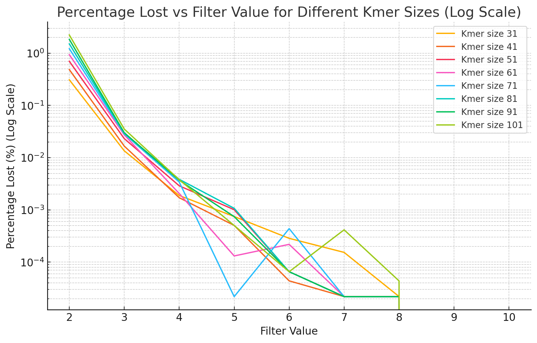
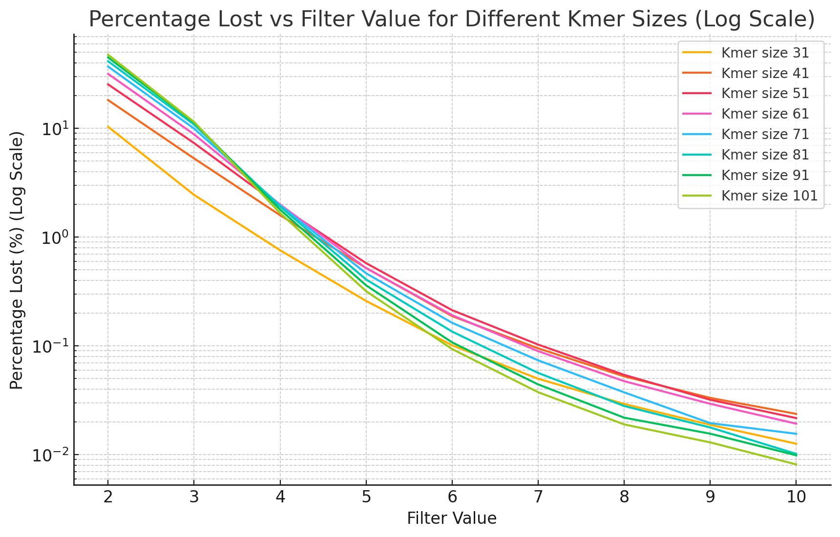
14.4.2 Super‑k‑mer threshold heuristic

We evaluate the super‑k‑mer abundance threshold by measuring how many k‑mers are dropped at each threshold (Figure 14.5). The proportion of lost k‑mers decreases exponentially with the threshold, and increases at lower coverage, larger k‑mer sizes, and higher error rates, mirroring classical k‑mer abundance filtering. To check that the lost k‑mers are erroneous rather than genomic, we count the genomic k‑mers absent from both KMC and KFC outputs across thresholds and k‑mer sizes (Figure 14.6). KFC drops a few more genomic k‑mers than KMC at low thresholds, but both methods converge as the threshold rises; on a dataset with a HiFi error rate (0.1%), KMC and KFC outputs match exactly. The super‑k‑mer-level threshold is therefore slightly more aggressive than a k‑mer-level threshold but conservative enough to preserve accuracy.

(a) HiFi dataset

(b) ONT dataset

Figure 14.5: Percentage of k‑mers lost by removing unique super‑k‑mers, as a function of the abundance threshold and k‑mer size. Left: simulated HiFi dataset with 100× coverage and 0.1% error rate. Right: simulated ONT dataset with 100× coverage and 1% error rate.

Figure 14.6: Amount of filtered genomic k‑mers by KFC and KMC according to the abundance threshold and k‑mer size, on a simulated 100× ONT E. coli dataset with 1% error rate.

14.5 Conclusion

This chapter introduced hyper‑k‑mers as a streaming, partitioned alternative to super‑k‑mers for large k‑mer sizes. By sharing each k - 1 base overlap between consecutive super‑k‑mers rather than duplicating it, hyper‑k‑mers asymptotically reach 4 bits per nucleotide, two thirds of the super‑k‑mer cost. This matches the closed-syncmer asymptote while hyper‑k‑mers remain a stand-alone k‑mer-set representation. We translated this representation to a practical k‑mer counter, KFC, which becomes both the fastest and the most memory-efficient tool past k \approx 200.

This compactness comes at two structural costs relative to super‑k‑mers. Each hyper‑k‑mer is now a pair of pointers into a shared pool of left and right parts rather than a contiguous string, so access carries one extra indirection per side along with the corresponding bookkeeping. The representation is also no longer self-contained at the k‑mer level: a given k‑mer can be covered by multiple hyper‑k‑mers when the sequence is revisited, so applications that require a unique representation must deduplicate explicitly. This last point parallels the limitation that the super‑k‑mer-level dictionary of Chapter 13 faces, and resolving it cleanly for either representation remains open work.

Compared to the static unitig-based representations of Chapter 2, which approach the 2-bit lower bound but require a separate counting pass and dissolve the per-minimizer partitioning, hyper‑k‑mers preserve both the streaming construction and the bucket structure that downstream indexes rely on for cache-friendly access and load balancing. The cost is the explicit deduplication step, and hyper‑k‑mers therefore sit structurally between super‑k‑mers and static SPSS representations.

Several directions remain open. The asymptotic 4 bits per nucleotide of hyper‑k‑mers is still twice the lower bound of 2 bits, and finding a representation that achieves this lower bound while keeping streaming construction is an open question. At the other end of the k‑mer size spectrum, hyper‑k‑mers do not scale well to small k, where the smaller minimizer size leaves many distinct hyper‑k‑mer contexts under each minimizer bucket and bucket scans dominate the cost. Lengths below 16 can be handled by a plain hash table on k‑mers themselves, but the range 17 to 63 is not well served by either approach and is a natural target for future work on dynamic linear representations. Finally, the current KFC algorithm discards k‑mers belonging to non-solid super‑k‑mers that share no minimizer with a solid super‑k‑mer, as discussed in Section 14.3. This heuristic is highly efficient in practice, but handling the corner case without losing performance would close the small accuracy gap with k‑mer-level filtering.

Bankevich, A., Bzikadze, A.V., Kolmogorov, M., Antipov, D., & Pevzner, P.A. (2022) Multiplex de bruijn graphs enable genome assembly from long, high-fidelity reads. Nature Biotechnology, 40, 1075–1081.

Benoit, G., Raguideau, S., James, R., Phillippy, A.M., Chikhi, R., & Quince, C. (2024) High-quality metagenome assembly from long accurate reads with metaMDBG. Nature Biotechnology, 42, 1378–1383.

Deorowicz, S., Debudaj-Grabysz, A., & Grabowski, S. (2013) Disk-based k-mer counting on a PC. BMC Bioinformatics, 14.

Deorowicz, S., Kokot, M., Grabowski, S., & Debudaj-Grabysz, A. (2015) KMC 2: fast and resource-frugal k-mer counting. Bioinformatics, 31, 1569–1576.

Dı́az-Domı́nguez, D., Leinonen, M., & Salmela, L. (2024) Space-efficient computation of k-mer dictionaries for large values of k. Algorithms Mol. Biol., 19, 14.

Edgar, R. (2021) Syncmers are more sensitive than minimizers for selecting conserved k-mers in biological sequences. PeerJ, 9, e10805.

Erbert, M., Rechner, S., & Müller-Hannemann, M. (2017) Gerbil: A fast and memory-efficient k-mer counter with GPU-support. Algorithms for Molecular Biology, 12.

Feng, X., Cheng, H., Portik, D., & Li, H. (2022) Metagenome assembly of high-fidelity long reads with hifiasm-meta. Nature Methods, 19, 671–674.

Kokot, M., Długosz, M., & Deorowicz, S. (2017) KMC 3: counting and manipulating k-mer statistics. Bioinformatics, 33, 2759–2761.

Marçais, G. & Kingsford, C. (2011) A fast, lock-free approach for efficient parallel counting of occurrences of k-mers. Bioinformatics, 27, 764–770.

Martayan, I., Robidou, L., Shibuya, Y., & Limasset, A. (2025) Hyper-k-mers: Efficient streaming k-mers representation. Research in computational molecular biology (RECOMB 2025). Springer Nature Switzerland.

Myers, G. (2023) FASTK: A fast K-mer counter for high-fidelity shotgun datasets. URL https://github.com/thegenemyers/FASTK.

Sereika, M., Kirkegaard, R.H., Karst, S.M., Michaelsen, T.Y., Sørensen, E.A., Wollenberg, R.D., & Albertsen, M. (2022) Oxford nanopore R10.4 long-read sequencing enables the generation of near-finished bacterial genomes from pure cultures and metagenomes without short-read or reference polishing. Nature Methods, 19, 823–826.

Shibuya, Y., Belazzougui, D., & Kucherov, G. (2022) Efficient Reconciliation of Genomic Datasets of High Similarity. 22nd International Workshop on Algorithms in Bioinformatics (WABI 2022). Schloss Dagstuhl – Leibniz-Zentrum für Informatik, pp. 14:1–14:14.