Appendix E — Proofs and experiments on fractional hitting sets
E.1 Useful lemmas
Lemma E.1 Assuming p is non-increasing with respect to w, 1 - (1 - p)^{w+1} \underset{w \to \infty}{=} f + o(1)
Proof. (1-p)^{w+1} = (1-p)^w - p (1-p)^w
- if p \underset{w \to \infty}{\longrightarrow} 0, p (1-p)^w \underset{w \to \infty}{\longrightarrow} 0
- otherwise p \ge c for some c > 0 since it is non-increasing, so p (1 - p)^w \le p (1 - c)^w \underset{w \to \infty}{\longrightarrow} 0
Therefore, (1-p)^{w+1} = (1-p)^w + o(1)
We use \widehat{\mathcal{S}} to denote the set of k‑mers containing a small m-mer.
Lemma E.2 Given two consecutive k‑mers W_0 and W_1, \Pr(W_0, W_1 \in \widehat{\mathcal{S}}) \underset{w \to \infty}{=} f + o(1)
Proof. \begin{aligned} \Pr(W_0, W_1 \in \widehat{\mathcal{S}}) & = 1 - \Pr(W_0 \notin \widehat{\mathcal{S}} \lor W_1 \notin \widehat{\mathcal{S}}) \\ & = 1 - \left[\Pr(W_0 \notin \widehat{\mathcal{S}}) + \Pr(W_1 \notin \widehat{\mathcal{S}}) - \Pr(W_0 \notin \widehat{\mathcal{S}} \land W_1 \notin \widehat{\mathcal{S}})\right] \\ & = 1 - 2 (1 - p)^w + (1 - p)^{w+1} = 1 - (1 - p)^w + o(1) \\ % \quad (\text{Lemma } \ref{lem-o1}) \\ & = f + o(1) \end{aligned}
Lemma E.3 p \underset{w \to \infty}{=} -\frac{1}{w} \ln(1 - f) + o(1/w)
Proof. Because of Proposition 17.1, we have p = 1 - (1 - f)^{1/w} and (1 - f)^{1/w} = \exp\left[\frac{1}{w} \ln(1 - f)\right] = 1 + \frac{1}{w} \ln(1 - f) + o(1/w)
E.2 Proof of Theorem 17.1
In order to upper bound the density, we follow the same approach as the one presented in (Zheng et al., 2020) (for the proof of theorem 7). As stated in (Zheng et al., 2020), the density is equivalent to the probability that a context c (that is, the string formed by two consecutive k‑mers) is charged, i.e. the two k‑mers of c have different minimizers. \begin{aligned} d & = \Pr_{c, h}(c \text{ is charged}) \\ & \le \Pr_{c, h}(c \text{ has duplicate } m\text{-mers}) + \Pr_{c, h}\left(c \text{ is charged}\ |\ \text{no duplicate } m\text{-mers}\right) \end{aligned}
Lemma E.4 (lemma 9 from (Zheng et al., 2020)) Assuming m > (3 + \varepsilon) \log_\sigma w, \Pr_{c, h}(c \text{ has duplicate } m\text{-mers}) = o(1 / w)
If c has no duplicate m-mers, the small m-mers are all distinct and each of them has the same probability to be minimal since h is random. Therefore, \Pr_{c, h}\left(c \text{ is charged}\ |\ \text{no duplicate } m\text{-mers}\right) = \mathbb{E}_{c, h}\left[\frac{M_{boundary}}{M_{total}}\right] where M_{boundary} denotes the number of boundary m-mers that are small and M_{total} denotes the total number of small m-mers in c.
Let x_0 denote the first m-mer of c and x_w denote the last one, \begin{aligned} \mathbb{E}_{c, h}\left[\frac{M_{boundary}}{M_{total}}\right] & = \mathbb{E}_{c, h}\left[\frac{\mathbf{1}_{x_0 \in \mathcal{S}} + \mathbf{1}_{x_w \in \mathcal{S}}}{M_{total}}\right] = 2 \cdot \mathbb{E}_{c, h}\left[\frac{\mathbf{1}_{x_0 \in \mathcal{S}}}{M_{total}}\right] \quad (\text{symmetry}) \\ & = 2 \cdot \mathbb{E}_{c, h}\left[1 / M_{total}\ |\ x_0 \in \mathcal{S}\right] \cdot \Pr(x_0 \in \mathcal{S}) \end{aligned}
Assuming x_0 is small, we have M_{total} = 1 + X with X \sim B(w, p), since each other m-mer of c has a probability p to be small. \mathbb{E}_{c, h}\left[1 / M_{total}\ |\ x_0 \in \mathcal{S}\right] = \mathbb{E}_{c, h}\left[\frac{1}{1 + X}\right] = \sum_{i = 0}^w \frac{1}{1 + i} \binom{w}{i} p^i (1-p)^{w-i}
Lemma E.5 \sum_{i = 0}^w \frac{1}{1 + i} \binom{w}{i} p^i (1-p)^{w-i} = \frac{1 - (1 - p)^{w+1}}{(w + 1) p}
Proof. \begin{aligned} & (w+1) p \sum_{i = 0}^w \frac{1}{1 + i} \binom{w}{i} p^i (1-p)^{w-i} = \sum_{i = 0}^w \frac{w+1}{1 + i} \frac{w!}{i! (w-i)!} p^{i+1} (1-p)^{w-i} \\ & = \sum_{i = 0}^w \frac{(w+1)!}{(i+1)! (w+1-(i+1))!} p^{i+1} (1-p)^{w+1-(i+1)} = \sum_{j = 1}^{w+1} \binom{w+1}{j} p^{j} (1-p)^{w+1-j} \\ & = 1 - (1-p)^{w+1} \end{aligned}
Finally, since \Pr(x_0 \in \mathcal{S}) = p, d \le 2 \cdot \frac{1 - (1 - p)^{w+1}}{w + 1} + o(1/w) = \frac{2 f}{w + 1} + o(1/w) % \quad (\text{Lemma } \ref{lem-o1})
E.3 Proof of Theorem 17.2
In this section, we assume that every k‑mer we work with contains a small m-mer.
Just as for the proof of Theorem 17.1, we still have
d \le \Pr_{c, h}(c \text{ has duplicate } m\text{-mers}) + \Pr_{c, h}\left(c \text{ is charged}\ |\ \text{no duplicate } m\text{-mers}\right)
and \begin{aligned} \Pr_{c, h}\left(c \text{ is charged}\ |\ \text{no duplicate } m\text{-mers}\right) & = \mathbb{E}_{c, h}\left[\frac{M_{boundary}}{M_{total}}\right] \\ &= 2 \cdot \mathbb{E}_{c, h}\left[1 / M_{total}\ |\ x_0 \in \mathcal{S}\right] \cdot \Pr(x_0 \in \mathcal{S}\ |\ W_1 \in \widehat{\mathcal{S}}) \end{aligned}
Lemma E.6 Assuming m > (3 + \varepsilon) \log_\sigma w, \Pr_{c, h}(c \text{ has duplicate } m\text{-mers}) = o(1 / w)
Proof. This proof is similar to the proof of lemma 9 from (Zheng et al., 2020). Let i, j \in \llbracket 0, w \rrbracket with i < j, \delta = j - i.
If \delta < m, \Pr(x_i = x_j) = \frac{\sigma^\delta}{\sigma^{m + \delta}} = \frac{1}{\sigma^m} = o(1/w^3)
If \delta \ge m, \begin{aligned} \Pr(x_i = x_j) & = \Pr(x_i = x_j\ |\ x_i, x_j \in \mathcal{S}) \Pr(x_i, x_j \in \mathcal{S}) + \Pr(x_i = x_j\ |\ x_i, x_j \notin \mathcal{S}) \Pr(x_i, x_j \notin \mathcal{S}) \\ & = \frac{\Pr(x_i, x_j \in \mathcal{S})}{p \cdot \sigma^m} + \frac{\Pr(x_i, x_j \notin \mathcal{S})}{(1-p) \sigma^m} \end{aligned} Because of Lemma E.2, \Pr(x_i, x_j \in \mathcal{S}) = \frac{p^2}{\Pr(W_0, W_1 \in \widehat{\mathcal{S}})} = \frac{p^2}{f + o(1)} \le p and \Pr(x_i, x_j \notin \mathcal{S}) \le \frac{(1-p)^2 \left[1 - (1-p)^{w-1}\right]}{\Pr(W_0, W_1 \in \widehat{\mathcal{S}})} = \frac{(1-p)^2 \left[1 - (1-p)^{w-1}\right]}{f + o(1)} \le (1-p)^2 Therefore, \Pr(x_i = x_j) \le \frac{p}{p \cdot \sigma^m} + \frac{(1-p)^2}{(1-p) \sigma^m} \le \frac{2}{\sigma^m} = o(1/w^3)
Thus \Pr_{c, h}(c \text{ has duplicate } m\text{-mers}) = \binom{w}{2} \times o(1/w^3) = o(1/w)
Assuming x_0 is small, the w next m-mers of c form a k‑mer, so we know that at least one of them is also small. Therefore, \begin{aligned} & \mathbb{E}_{c, h}\left[1 / M_{total}\ |\ x_0 \in \mathcal{S}\right] = \mathbb{E}_{c, h}\left[\frac{1}{1 + X}\ |\ X \ge 1\right] = \frac{1}{\Pr(X \ge 1)} \sum_{i = 1}^w \frac{1}{1 + i} \binom{w}{i} p^i (1-p)^{w-i} \\ & = \frac{1}{f} \left[\frac{1 - (1 - p)^{w+1}}{(w + 1) p} - (1 - p)^w\right] = \frac{1}{f} \left[\frac{f + o(1)}{(w + 1) p} - (1 - f)\right] % \quad (\text{Lemma } \ref{lem-wolfram} \text{ and } \ref{lem-o1}) \end{aligned}
What’s more, \Pr(x_0 \in \mathcal{S}\ |\ W_1 \in \widehat{\mathcal{S}}) = \frac{\Pr(x_0 \in \mathcal{S})}{\Pr(W_1 \in \widehat{\mathcal{S}})} = \frac{p}{f}.
Hence, \begin{aligned} d & \le \frac{2 p}{f^2} \left[\frac{f + o(1)}{(w + 1) p} - (1 - f)\right] + o(1/w) = \frac{2}{f (w+1)} - \frac{2 (1 - f) p}{f^2} + o(1/w) \\ & = \frac{2}{f (w+1)} + \frac{2 (1 - f) \ln (1 - f)}{f^2 w} + o(1/w) \\ % \quad (\text{Lemma } \ref{lem-eqp}) \\ & = 2 \cdot \frac{f + (1 - f) \ln (1 - f)}{f^2 (w+1)} + o(1/w) \end{aligned}
E.4 Proof of Theorem 17.3
In order to compute the proportion of maximal super‑k‑mers, we adapt the proof of theorem 4 from (Pibiri et al., 2023).

First, we introduce a similar Markov chain representing the position X of the small minimizer in the k‑mer, with an extra state \varnothing when there is no small minimizer.
We reuse the following notations introduced in (Pibiri et al., 2023):
- P_{lr} is the proportion of left-right-max (i.e. maximal) super‑k‑mers
- P_l is the proportion of left-max super‑k‑mers
- P_r is the proportion of right-max super‑k‑mers
- P_n is the proportion of non-max super‑k‑mers
\forall i \in \llbracket 1, w-1 \rrbracket, \Pr(\text{first } X = i) = \Pr(X = 1) \cdot \frac{f}{w} P_{lr} + P_r = \Pr(X = w) = \Pr(\text{first } X = w) = 1 - \sum_{i=1}^{w-1} \Pr(\text{first } X = i) = 1 - \Pr(X = 1) \cdot f \cdot (1 - 1/w) P_{lr} + P_l = \Pr(\text{last } X = 1) = \Pr(X = 1) + \Pr(\text{first } X = 1) = \Pr(X = 1) \cdot (1 + f/w) By symmetry, P_l = P_r, so 1 - \Pr(X = 1) \cdot f \cdot (1 - 1/w) = \Pr(X = 1) \cdot (1 + f/w)
Therefore, \Pr(X = 1) = \frac{1}{1 + f} and \Pr(X = w) = 1 - \frac{f}{1 + f} \left(1 - \frac{1}{w}\right) = \frac{1 + f/w}{1 + f}
What’s more, 1 + P_{lr} = P_{lr} + P_l + P_{lr} + P_r + P_n = 2 \cdot \Pr(X = w) + P_n
so P_{lr} = P_n + 2 \cdot \Pr(X = w) - 1 = P_n + \frac{1 - f(1 - 2/w)}{1 + f} \text{ and } P_l = P_r = \Pr(X = w) - P_{lr} = \frac{f(1 - 1/w)}{1 + f} - P_n
\begin{aligned} P_n & = \Pr(\text{first } X \neq w) \cdot \Pr(\text{last } X \neq 1) = \Pr(X = 1) \cdot f \cdot (1 - 1/w) \cdot \left[1 - \Pr(X = 1) \cdot (1 + f/w)\right] \\ & = \left(1 - \frac{1}{w}\right) \cdot \frac{f}{1 + f} \cdot \left[1 - \frac{1 + f/w}{1 + f}\right] = \left(1 - \frac{1}{w}\right) \cdot \frac{f}{1 + f} \cdot \frac{f (1 - 1/w)}{1 + f} = \left[\left(1 - \frac{1}{w}\right) \frac{f}{1 + f}\right]^2 \end{aligned}
Thus P_l = P_r = \left[\left(1 - \frac{1}{w}\right) \frac{f}{1 + f}\right] \left[1 - \left(1 - \frac{1}{w}\right) \frac{f}{1 + f}\right]
and P_{lr} = \left[\left(1 - \frac{1}{w}\right) \frac{f}{1 + f}\right]^2 + \frac{1 - f(1 - 2/w)}{1 + f}
E.5 Proof of Theorem 17.4
This proof generalizes the proof of Theorem 17.1 when the minimizers are selected from a UHS \mathcal{U} with density d_{\mathcal{U}}.
First, because of independence, we have \Pr(x_0 \in \mathcal{S} \cap \mathcal{U}) = \Pr(x_0 \in \mathcal{S}) \cdot \Pr(x_0 \in \mathcal{U}) and \Pr(|\mathcal{S} \cap \mathcal{U} \cap c| = i) = \sum_{n \ge i} \Pr(|\mathcal{U} \cap c| = n) \Pr(|\mathcal{S} \cap \mathcal{U} \cap c| = i\ |\ |\mathcal{U} \cap c| = n)
The main change of the proof lies in the bound on the expectation: \begin{aligned} \mathbb{E} & \left[\frac{1}{|\mathcal{S} \cap \mathcal{U} \cap c|}\ |\ x_0 \in \mathcal{S} \cap \mathcal{U}\right] = \sum_{i=0}^w \frac{1}{i+1} \Pr\left(|\mathcal{S} \cap \mathcal{U} \cap c| = i+1\ |\ x_0 \in \mathcal{S} \cap \mathcal{U}\right) \\ & = \sum_{i=0}^w \frac{1}{i+1} \sum_{n=i}^w \Pr(|\mathcal{U} \cap c| = n+1\ |\ x_0 \in \mathcal{U}) \Pr(|\mathcal{S} \cap \mathcal{U} \cap c| = i+1\ |\ |\mathcal{U} \cap c| = n+1, x_0 \in \mathcal{S} \cap \mathcal{U}) \\ & = \sum_{n=0}^w \Pr(|\mathcal{U} \cap c| = n+1\ |\ x_0 \in \mathcal{U}) \sum_{i=0}^n \frac{1}{i+1} \Pr(|\mathcal{S} \cap \mathcal{U} \cap c| = i+1\ |\ |\mathcal{U} \cap c| = n+1, x_0 \in \mathcal{S} \cap \mathcal{U}) \\ & = \sum_{n=0}^w \Pr(|\mathcal{U} \cap c| = n+1\ |\ x_0 \in \mathcal{U}) \sum_{i=0}^n \frac{1}{i+1} \Pr(|\mathcal{S}| = i+1\ |\ x_0 \in \mathcal{S}, |W| = n) \\ & = \sum_{n=0}^w \Pr(|\mathcal{U} \cap c| = n+1\ |\ x_0 \in \mathcal{U}) \cdot \frac{1 - (1-p)^{n+1}}{(n+1) p} \\ % \quad (\text{Lemma } \ref{lem-wolfram}) \\ & \le \sum_{n=0}^w \Pr(|\mathcal{U} \cap c| = n+1\ |\ x_0 \in \mathcal{U}) \cdot \frac{f + o(1)}{(n+1) p} % \quad (\text{Lemma } \ref{lem-o1}) \end{aligned}
Therefore, using the same arguments as in the proof of Theorem 17.1, we obtain \begin{aligned} d_{\mathcal{S} \cap \mathcal{U}} & \le 2 \cdot \Pr(x_0 \in \mathcal{S} \cap \mathcal{U}) \cdot \mathbb{E}\left[\frac{1}{|\mathcal{S} \cap \mathcal{U} \cap c|}\ |\ x_0 \in \mathcal{S} \cap \mathcal{U}\right] + o(1/w) \\ & \le 2 \cdot \Pr(x_0 \in \mathcal{U}) \cdot \Pr(x_0 \in \mathcal{S}) \sum_{n=0}^w \Pr(|\mathcal{U} \cap c| = n+1\ |\ x_0 \in \mathcal{U}) \cdot \frac{f}{(n+1) p} + o(1/w) \\ & = f \cdot 2 \cdot \Pr(x_0 \in \mathcal{U}) \sum_{n=0}^w \frac{1}{n+1} \Pr(|\mathcal{U} \cap c| = n+1\ |\ x_0 \in \mathcal{U}) + o(1/w) \\ & = f \cdot d_{\mathcal{U}} + o(1/w) \end{aligned}
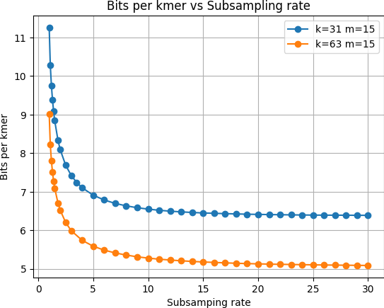
E.6 Additional figures